
Statistics notes
z-test, t-test, ANOVA and chi-squared tests, binomial distribution
Variance
Descriptive
- SD: Standard Deviation, σ²
- $s^2_n=\frac{1}{n}\sum(x_i - \bar{x})^2$
- Bessel’s correction
- $s^2=s^2_n\frac{n}{n-1}=\frac{1}{n-1}\sum(x_i - \bar{x})^2$
Inferential
- SE: Standard Error
- $SE_{\bar{x}} = \frac{s}{\sqrt{n}}$
- s2 is an estimation of σ2 the variance of the population.
- The higher the number of elements of the sample, the lower the SE.
Margin of error
\[ME = \pm z^* \cdot SE = \pm z^* \cdot\frac{\sigma}{\sqrt{n}}\]Types of tests
| degrees of freedom | Obvjective | Conditions | Formula | |
|---|---|---|---|---|
| One sample | ||||
| z-test | - | $\bar{x}$ vs μ | - Normal distribution -σ and μ are known |
$z=\frac{\bar{x}-\mu}{\frac{\sigma}{\sqrt{n}}}$ |
| t-test | n-1 | $\bar{x}$ vs μ | - Normal distribution -σ unknown -μ known |
$t=\frac{\bar{x}-\mu}{\frac{s}{\sqrt{n}}}$ |
| Two sample | ||||
| t-test independent samples |
df1 + df2 = n1 + n2 − 2 | - σ1,σ2 unknown - σ1 ∼ σ2 |
- Normal distribution -$s^2_p=\frac{(n_1-1)s^2_1+(n_2-1)s^2_2}{n_1+n_2-2}$ |
$t=\frac{\bar{x}_1-\bar{x}_2}{s_p\sqrt{\frac{1}{n_1}+\frac{1}{n_2}}}$ |
| t-test dependent samples |
n − 1 | - σ1,σ2 unknown - σ1 ∼ σ2 di = x1i − x2i |
- Normal distribution - 2 dependent samples (pre-treatment, post-treatment) $s_d= \sqrt{\frac{\sum(d_i-\bar{d})^2}{n}}$ |
$t=\frac{\bar{d}}{\frac{s_d}{\sqrt{n}}}$ |
| Three or more samples | ||||
| One way ANOVA |
dfbtw = k − 1 dfw = N − K N = ∑nk N = number of elements k= number of groups |
- diff 3 or more population means | - Normal distribution -s12, s22 sample variances |
$F= \frac{\frac{SS_{btw}}{df_{btw}}}{\frac{SS_w}{df_w}} = \frac{\sum n_k(\bar{x}_k-\bar{x}_G)^2/(K-1)}{\sum_{k=1}^{K}\sum_{i=1}^{n_k}(x_i-\bar{x}_k)^2/(N-K)}$ |
ANOVA
\[MS_{between}=\frac{SS_{btw}}{df_{btw}}= \frac{\sum_{k=1}^{K}n_k(\bar{x}_k-\bar{x}_G)^2}{K-1}\] \[MS_{within}= \frac{SS_w}{df_w} = \frac{\sum_{k=1}^{K}\sum_{i=1}^{n_k}(x_i-\bar{x}_k)^2}{N-K}\]for N the total number of elements and K the total number of groups.
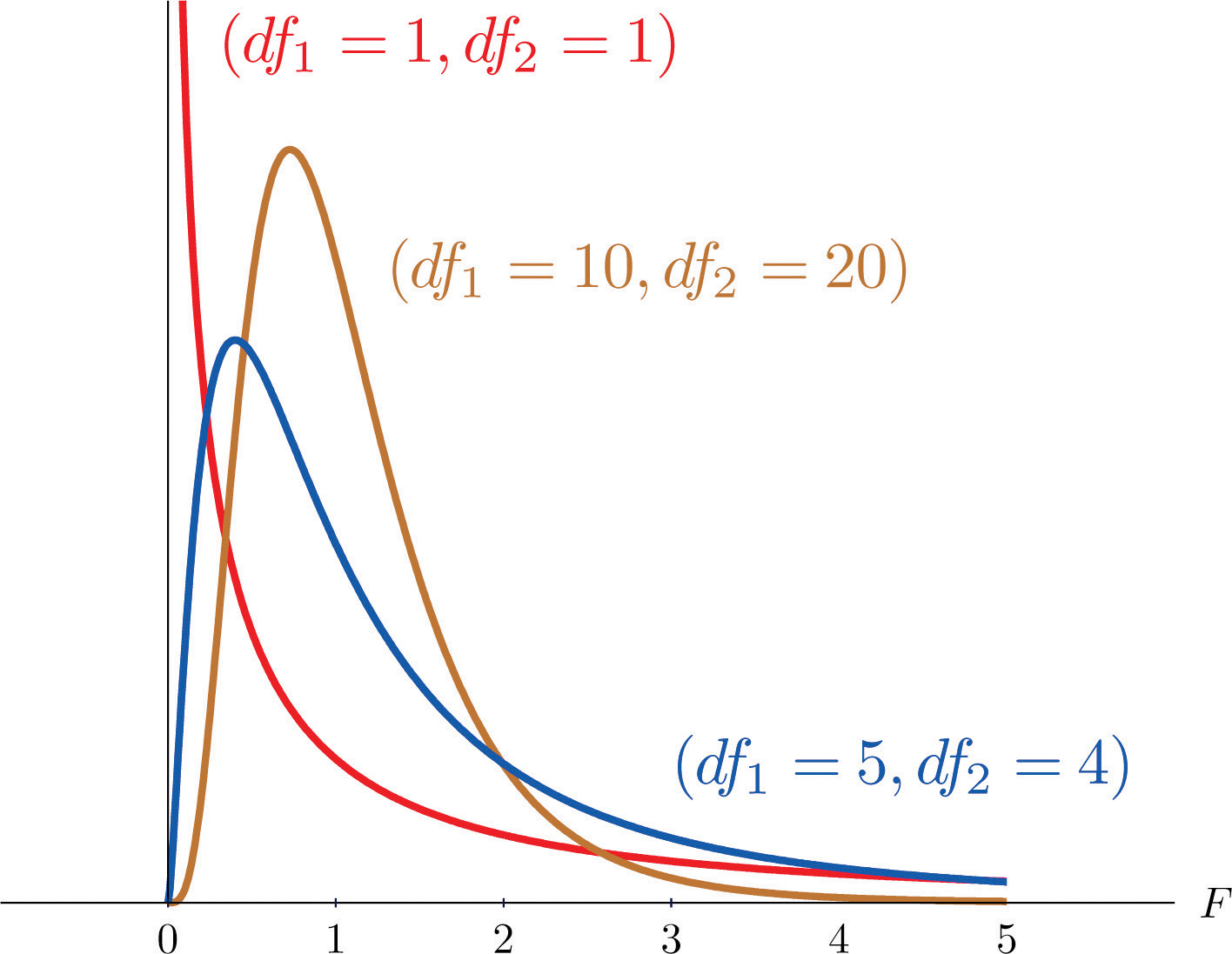
\[F= \frac{\frac{SS_{btw}}{df_{btw}}}{\frac{SS_w}{df_w}} = \frac{\sum n_k(\bar{x}_k-\bar{x}_G)^2/(K-1)}{\sum_{k=1}^{K}\sum_{i=1}^{n_k}(x_i-\bar{x}_k)^2/(N-K)}\]F-statistic characteristics
- ∀ > 0
-
- skewed
Cohen’s d for multiple comparisons -> effect size —————————————————-
\[d=\frac{\bar{x}_1-\bar{x}_2}{\sqrt{MS_{within}}}=\frac{\bar{x}_1-\bar{x}_2}{\sqrt{\frac{\sum(x_i-\bar{x}_k)^2}{N-k}}}\]Eta-squared η2
η2 : proportion of total variation due to between group differences (explained variation)
\[\eta^2=\frac{SS_{between}}{SS_{total}}\]Correlation coefficient (Pearson’s r)
For a population
\(\rho_{X,Y}= \frac{cov(X,Y)}{\sigma_X\cdot \sigma_Y}\) Pearson’s correlation coefficient when applied to a population is commonly represented by the Greek letter ρ and may be referred to as the population correlation coefficient or the population Pearson correlation coefficient.
Where cov(X, Y)=E[(X − μX)(Y − μY)] for E[X] the expected value of X or mean of X.
| When | ρ | =1 this means that data lies in perfect line. |
For a sample
Pearson’s correlation coefficient is represented as r when applied to a sample and it is called sample correlation coefficient or sample Pearson correlation coefficient.
\[r= \frac{\sum^n_{i=1}(x_i-\bar{x})(y_i - \bar{y})}{\sqrt{\sum^n_{i=1}(x_i-\bar{x})^2}\sqrt{\sum^n_{i=1}(y_i-\bar{y})^2}}\]Hypothesis testing
\[\begin{align*}H_o:&\rho=0 \\ H_A: &\rho<0 \\ &\rho >0 \\ &\rho\neq0 \end{align*}\]Student’s t-distribution
\[t=r\sqrt{\frac{n-2}{1-r^2}}\]Which is a t-distribution with d**f = n − 2, for n the number of elements in the sample.
Regression
Linear regression: $\hat{y}=a+bx$
\[b = \frac{\sum_{i=1}^n(x_i-\bar{x})(y_i-\bar{y})}{\sum_{i=1}^n(x_i-\bar{x})^2} = r \frac{s_y}{s_x}\]SD: how far values will fall from the regression line.
SD of the estimate = $\sqrt{\frac{\sum(y-\hat{y})^2}{n-2}}$
$residuals=\sum{(y_i -\hat{y_i})^2}$
Line of best fit: minimizes residuals

Confidence interval (CI) ————————
Population
- β0: population yint
- β1: population slope
Sample
- a : sample yint
- b : sample slope
Hypothesis testing
\[\begin{align*}H_o:&\beta_1=0 \\ H_A: &\beta_1\neq0 \\ &\beta_1>0 \\ &\beta_1<0 \end{align*}\]d**f = n − 2, for n the number of elements in the sample.
χ2 test for independence
\[\chi^2 = \sum_{i=1}^n{\frac{(f_{oi} - f_{ei})^2}{f_{ei}}}\]- ∀ χ2 > 0
- ∀ one-directional test
- χcri**t2
1 variable with ≠ responses
d**f = n − 1
2 or more variables
d**f = (nrow**s − 1)(ncol**s − 1) for N the number of categories
\[f_{ei} = \frac{(column\; total)(row\,total)}{grand \,total}\]Binomial distribution
- Propability: $P(X=r)= \binom {n} {r}p^r(1-p)^{n-r}$
- Mean: μ = n**p
- Variance: σ2 = n**p(1 − p)
- Standard deviation $s = \sqrt{np(1-p)}$
- $SE = \sqrt{\frac{p(1-p)}{n}}$
Confidence Interval (CI)
$\hat{p}=\frac{x}{N}$
$SE = \sqrt{\frac{\hat{p}(1-\hat{p})}{N}}$
A distribution can be considered normal if $N\hat{p}>5$ or $N(1-\hat{p})>5$
Margin of error \(m = z\cdot SE = z\cdot\sqrt{\frac{\hat{p}(1-\hat{p})}{N}}\)
Pooled Standard Error (S**Ep)
Comparing two samples
Xcontrol, Xexperimen**t, Ncontrol, Nexperimen**t
\(\hat{p}_{p}= \frac{X_{control}+X_{exp}}{N_{control}+N_{exp}}\) Pooled Standard Error (S**Ep) \(SE_{p}= \sqrt{\hat{p}_p\cdot(1-\hat{p}_p)\left(\frac{1}{N_{control}}+\frac{1}{N_{exp}}\right)}\) \(\hat{d}=\hat{p}_{exp}-\hat{p}_{control}\)
\[\begin{align*}&H_0:& d=0 &\rightarrow \hat{d}\sim N(0,SE_{p}) \\ &H_A:& d\neq 0 & \rightarrow Reject\; Null:|\hat{d}| > z^* SE_{p}\end{align*}\]

References: ———–